As this is the inaugural issue of the found-this-week series, I’ll briefly note my motivation and inspiration. The title of this series is an overt nod to the famous series This Week’s Finds written by the inimitable John Baez. I have learned a great deal from that series and his book on gravity, and have the utmost admiration for Baez’ abilities as a physicist and communicator. It is my hope that this series will be found useful by some, insightful by at least a few, and accessible by many. All feedback is welcome, and thank you in advance for bearing with me as I develop these posts.

Algebraic and Geometric Equivalence of Tangent Vectors

As will likely come up in future posts, I’m thoroughly enjoying Modern Differential Geometry for Physicists by Chris Isham. He develops formalism and intuition without sacrificing rigor, all while carrying a conversational tone. See my reference review for more. ¹

Most students of physics or calculus are generally familiar with the notion of a tangent vector. This concept becomes more nuanced, of course, when the ambient space is generalized from $\mathbb{R}^n$ to a manifold $\mathcal{M}$ of dimension $n$. Isham takes an unusual approach to formalizing the tangent vector concept by introducing two seemingly-different definitions (either of which are common among the relativity literature) and then formally proving their equivalence (done nowhere in the literature). I appreciated the demonstration of equivalence, and will sketch it below.

Tangent Vectors Geometrically

Isham first introduces tangent vectors in the familiar, geometric manner. If we let $\gamma_1(\lambda)$ and $\gamma_2( \lambda)$ be curves passing through a point $p$ on a patch of the manifold $\mathcal{M}$ such that $\gamma_1(\lambda=0) = \gamma_2(\lambda=0) = p$, then it is natural to define the tangent vector $v_p$ at $p$ as an equivalence class of curves, denoted $\left[\gamma\right]$, where the equivalence criteria is defined by sharing the tangent vector $v_p$:

$$\left. \frac{d x^{\mu}}{d \lambda} (\gamma_1(\lambda)) \right|_{\lambda=0} = v_p = \left. \frac{d x^{\mu}}{d \lambda} (\gamma_2(\lambda)) \right|_{\lambda=0}$$

The tangent space $T_p \mathcal{M}$ can then be defined as the set of all tangent vectors at the point $p$, or the set of all equivalence classes of curves at the point $p$.

Tangent Vectors Algebraically

The algebraic approach begins with the concept of a derivation, or directional derivative, $v$ as a map that is both linear and obeys the Leibniz rule. By thinking of the smooth functions on the manifold $C^{\infty}(\mathcal{M})$ as a ring over $\mathbb{R}$, we can define the map $v: C^{\infty}(\mathcal{M}) \to \mathbb{R}$ as:

$$v(f) \equiv \left. \frac{df\left( \gamma(\lambda) \right)}{d\lambda} \right|_{\lambda=0} \quad\text{ where }\quad \left[\gamma\right] = v$$

By linear, we mean that for any $f, g \in C^{\infty}(\mathcal{M})$ and $r, s \in \mathbb{R}$, we have $v(rf + sg) = rv( f) + sv(g)$, and by Leibniz rule we mean $v(fg) = f(p)v(g) + g(p)v(f)$. The set of all derivations at a point $p$ is denoted $D_p \mathcal{M}$.

Equivalence of Definitions

Isham shows that these two definitions of the tangent space, $T_p \mathcal{M}$ and $D_p \mathcal{M}$, are equivalent by proving that the natural map between them $\iota$ is, in fact, an isomorphism, where $\iota: T_p\mathcal{M} \to D_p\mathcal{M}$ is defined as:

$$\iota(v)(f) \equiv \left. \frac{df \left(\gamma\left(\lambda\right)\right) }{d\lambda} \right|_{\lambda=0}$$

To show that $\iota$ is an isomorphism, Isham demonstrates that it is both injective (one-to-one) and surjective (onto). To show injectivity, assume that $\iota(\left[\gamma_1\right]) = \iota(\left[\gamma_2\right])$, then we must have

$$\left. \frac{df \left(\gamma_1\left(\lambda\right)\right) }{d\lambda} \right|_{\lambda=0}$$

The above shows that both $\gamma_1$ and $\gamma_2$ are tangent at $p$, which implies that they are, in fact, equivalent. Therefore $\left[\gamma_1\right] = \left[\gamma_2\right]$, and $\iota$ is injective. To show that $\iota$ is surjective we choose an element $v$ of the range $D_p\mathcal{M}$ and define a curve $\gamma_v$ such that $\gamma_v(0)=p$ and $v(x^{\mu})=\frac{d}{d\lambda}x^{\mu}\circ\gamma(\lambda)|_{\lambda=0}$. Recall that we can expand a tangent vector as $v_p$ in terms of derivatives of a coordinate system $x^{\mu}$ as $v = v^{\mu}\partial_{\mu}$ and therefore $v(f) = v^{\mu} \partial_{\mu} f = \frac{d}{d\lambda} x^{\mu} \circ \gamma_v |_{\lambda=0} \partial_{\mu} f$. But Isham shows:

$$\begin{align} \left. \frac{d}{d\lambda} f\circ \gamma_v \right|_{\lambda=0} &= \left. \frac{d}{d\lambda}(f \circ \phi^{-1} \circ \phi \circ \gamma_v) \right|_{\lambda=0} \\\\ &= \sum_{\mu} \left. \frac{\partial}{\partial u^{\mu}} (f\circ \phi^{-1}) \right|_{\phi(p)} \left. \frac{d}{d\lambda} u^{\mu} (\phi \circ \gamma_v) \right|_{\lambda=0} \\\\ &= \sum_{\mu} \left(\frac{\partial}{\partial x^{\mu}}\right)_{p} f \left. \frac{d}{d\lambda} x^{\mu} \circ \gamma_v(\lambda) \right|_{\lambda=0} = v(f) \end{align}$$

Since $\frac{d}{d\lambda} f \circ \gamma_v |_{\lambda=0} = v(f)$, then $\left[\gamma_v\right](f) = v(f)$ and therefore $\iota$ is surjective. This completes the proof, and we can robustly conclude that the geometric and algebraic pictures are formally equivalent! We are then free to use either where convenient.

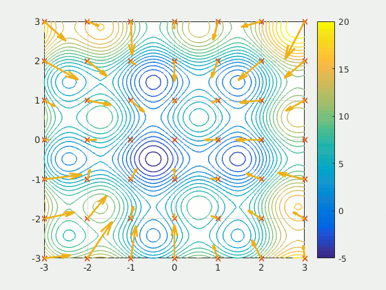
Swarms of Searching Particles

During a recent talk the subject of optimization arose in the context of gravitational wave detection. ² Though interested in the application (my present research overlaps heavily with GW detection), the general concept of particle swarm optimization (PSO) captured my attention.

This optimization method involves an initial distribution of $m$ particles $\{x^{\mu}_{k}\}$ in the $n$-dimensional parameter space $\mathcal{M}$ of some measure of quality $f: \mathcal{M} \to \mathbb{R}$, where $\mu = 1, \dots, n$ refers to the coordinate in $\mathcal{M}$ and $k = 1, \dots, m$ refers to the particle number. Each particle is initialized with some velocity, and the velocity is updated throughout each iteration of the algorithm. Interestingly, the particles are not computing local gradients, rather, their velocities are updated using a randomized combination of local (nearest-neighbors-in-swarm) and global (all-swarm) information. The iteration rule can be summarized broadly by the equation below.

$$\begin{align} v^{\mu}_{k}(t) &= c_0 v^{\mu}_{k}(t - \Delta t) \\\\ &+ c_1 r_1 \left[\eta^{\mu}_k(t - \Delta t) - x^{\mu}_k(t - \Delta t)\right] \\\\ &+ c_2 r_2 \left[\zeta^{\mu}(t - \Delta t) - x^{\mu}_k(t - \Delta t)\right] \end{align}$$

Where the variable $\eta^{\mu}_k$ represents the best known position of the local neighbors of particle $k$ and the variable $\zeta^{\mu}$ represents the best known position of the entire swarm (also called the global best). The term best here refers to the type of optimization, in our example we would maximizing our quality function $f$, so for example $\zeta^{\mu}$ is the position in the swarm that corresponds to the larges value of $f$. When the velocity updates, the algorithm is essentially trying to mix three things:

1. The previous direction of the particle
2. The direction towards the known, local optimum
3. The direction toweards the known, global optimum

For further reading, the PSO algorithm has been studied extensively in general.³ PSO has also been used in a variety of scientific fields, such as gravitational wave analysis,⁴ and has even been used in industry settings, such as financial portfolio optimization.⁵